Synthetic Clusters
Prerequisites
Add the Congrads package to the current Colab notebook environment and install it.
Import the necesary functions and classes.
Define utility functions for plotting and other.
Define custom classes.
Before starting with the general training procedure, we fix the randomizer seeds and get the device on which we are training our model:
We have a built-in Seeder class that will pseudo-randomly fix the seeds of random number generators, Numpy and PyTorch.
If there is a GPU available, use it. Otherwise fall back to CPU.
Problem description
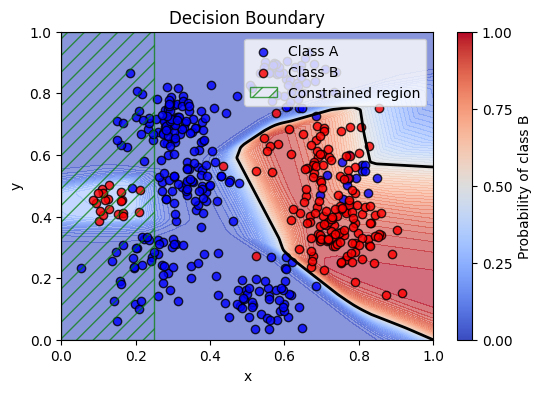
In this second example, the goal is to make a binary classification on some noisy training examples.
We aim to train a classifier that respects constraints put on the network. More specifically, for a certain part in the domain we want to enforce a high probability for class A.
Mathematically: \(x \le 0.25\), then \(P(\text{Blue}) \ge 0.7\)

Dataset
For this example we will use the built-in SyntheticClusters dataset and we will split the dataset into training, validation and test sets using another built-in utility function.
# Load and preprocess data
dataset = SyntheticClusters(
    cluster_centers=[
        (0.3, 0.70),
        (0.25, 0.25),
        (0.13, 0.45),
        (0.35, 0.5),
        (0.67, 0.6),
        (0.80, 0.55),
        (0.75, 0.35),
        (0.55, 0.15),
        (0.6, 0.85),
    ],
    cluster_sizes=[100, 50, 20, 50, 50, 15, 100, 50, 50],
    cluster_std=[0.06, 0.07, 0.04, 0.06, 0.07, 0.04, 0.07, 0.06, 0.06],
    cluster_labels=[0, 0, 1, 0, 1, 0, 1, 0, 0],
)
loaders = split_data_loaders(
    dataset,
    loader_args={"batch_size": 100, "shuffle": True},
    valid_loader_args={"shuffle": False},
    test_loader_args={"shuffle": False},
)
Network
For this example we will use a slightly modified fully connected MLPNetwork with a softmax layer on the output. For this use the prepared MLPNetworkWithSoftmax network.
# Instantiate an MLPNetworkWithSoftmax, configure the parameters
network = MLPNetworkWithSoftmax(n_inputs=2, n_outputs=2, n_hidden_layers=3, hidden_dim=50)

# Push the network to the current device
network = network.to(device)
Descriptor
Now that we have the dataset and the network defined, we can set up an important feature in the Congrads toolbox, called the Descriptor.
Please assign tags to all inputs and all outputs. Flag the input tags as constant.
Example:
descriptor = Descriptor()
descriptor.add("input", "t", 0, constant=True)   # Assigns tag 't' to input data tensor column 0
Refer to the descriptor documentation for more information.
# Instantiate descriptor
descriptor = Descriptor()

# Add constant tags for the inputs
descriptor.add("input", "x", 0, constant=True)
descriptor.add("input", "y", 1, constant=True)

# Add variable tags for the outputs
descriptor.add("output", "ProbA", 0)
descriptor.add("output", "ProbB", 1)
Constraints
With the help of the descriptor, we can easily reference certain parts of the neural network, and so we can now define our constraints.
We have numerous pre-defined constraints available that allow a variety of options. Some examples:
ScalarConstraintallows enforcing that data referenced by a tag should be above or below a certain scalar valueImplicationConstraintallows conditionally enforcing constraints. If constraint X satisfies, then enforce constraint Y.
In this example, we want to train a classifier that respects constraints put on the network. More specifically, for a certain part in the domain we want to enforce a high probability for class A.
The objective: \(x \le 0.25\), then \(P(\text{Blue}) \ge 0.7\)
# Assign descriptor to constraint base
Constraint.descriptor = descriptor

# Assign device to constraint base
Constraint.device = device

# Define constraints
constraints = [
    ImplicationConstraint(
        head=ScalarConstraint("x", "<=", 0.25),
        body=ScalarConstraint("ProbA", ">=", 0.7),
    ),
]
Loss and optimizer
For this example, we will use a modified loss function that will first convert the predicted probabilities back into logits, and then apply an NLLLoss function to it. Use the prepared NNLLossFromProb for this.
We will stick to the Adam optimizer for this example.
# Instantiate loss criterion
criterion = NNLLossFromProb()

# Instantiate optimizer
optimizer = Adam(network.parameters(), lr=0.001)
Metric manager
To allow keeping track of constraint satisfaction rates for each individual constraints, as well as the losses and possibly other metrics, we instantiate a metric manager.
# Initialize metric manager
metric_manager = MetricManager()
Core
The CongradsCore is the brain of the toolbox. It orchestrates the functionality of all previously created objects, integrating descriptors, constraints, and optimization strategies to perform constraint-guided gradient descent. Essentially, it manages the full training or evaluation pipeline: preparing input and output tensors, applying constraints, computing gradients, updating model parameters, and generating predictions in a coordinated manner.
First, we define a callback that handles plotting per epoch.
Refer to the Congrads documentation for more info.
callback_manager = CallbackManager()

class PlottingCallback(Callback):
    def on_epoch_end(self, data, ctx):
        clear_output(wait=True)
        plot_decision_boundary(network, dataset)
        plt.show()
        plt.close()

callback_manager.add(PlottingCallback())
<CallbackManager callbacks=['PlottingCallback'] ctx_keys=[]>
# Instantiate core
core = CongradsCore(
    descriptor=descriptor,
    constraints=constraints,
    dataloader_train=loaders[0],
    dataloader_valid=loaders[1],
    dataloader_test=loaders[2],
    network=network,
    callback_manager=callback_manager,
    criterion=criterion,
    optimizer=optimizer,
    metric_manager=metric_manager,
    device=device,
    enforce_all=True,
)
Finally, we can start training by running the core.fit(...) function. This function allows setting the maximum epochs and callback functions and will start the training process.
# Start training
core.fit(max_epochs=350)
Epoch: 100%|██████████| 350/350 [03:12<00:00, 1.82it/s]